Understanding the EM Algorithm | Part I

The EM algorithm is very straightforward to understand with one or two proof-of-concept examples. However, if you really want to understand how it works, it may take a while to walk through the math. The purpose of this article is to establish a good intuition for you, while also provide the mathematical proofs for interested readers. The codes for all the examples mentioned in this article can be found at https://github.com/mistylight/Understanding_the_EM_Algorithm.

Hello world: Two coins

Let’s get started with a simple example from [1].

Warm-up

Suppose you have 2 coins A and B with unknown probability of heads, $p_A$ and $p_B$.

In order to estimate $p_A$ and $p_B$, you did an experiment consisting of 5 trials. In each trial, you pick either coin A or B, and then toss it for 10 times.

Suppose this is what you get from your experiment:

Trial ID	Coin	Result	#heads / #tails
#1	B	HTTTHHTHTH	5/5
#2	A	HHHHTHHHHH	9/1
#3	A	HTHHHHHTHH	8/2
#4	B	HTHTTTHHTT	4/6
#5	A	THHHTHHHTH	7/3

How do we estimate $p_A$ and $p_B$ from this data? That’s quite straightforward. For coin A, it was tossed in trial #2, #3, #5, therefore we sum up the head count and divide them by the total number of tosses in these three trials:

$p_A=\dfrac{9+8+7}{10+10+10}=0.8$

The same logic applies to coin B, which was tossed in trial #1 and #4:

$p_B = \dfrac{5+4}{10+10} = 0.45$

To sum up, in order to infer $p_A$ and $p_B$ from a group of trials, we follow the two steps below:

💡 Algorithm 1: Maximum-Likelihood Estimation (MLE) — Infer $p_A$ and $p_B$ from complete data.

1. Partition all trials into 2 groups: the ones with coin A, and the ones with coin B;
2. Compute $p_A$ as the total number of head tosses divided by the total number of tosses across the first group, and $p_B$ as that of the second group.

Challenge: From MLE to EM

Now let’s consider a more challenging scenario: You forgot to take down which coin was tossed at each trial, so now your data looks like this:

Trial ID	Coin	Result	#heads / #tails
#1	Unknown	HTTTHHTHTH	5/5
#2	Unknown	HHHHTHHHHH	9/1
#3	Unknown	HTHHHHHTHH	8/2
#4	Unknown	HTHTTTHHTT	4/6
#5	Unknown	THHHTHHHTH	7/3

E-Step

How do we estimate $p_A$ and $p_B$ from this incomplete data? The main problem is that the first step of Algorithm 1 no longer works — We cannot know for sure whether a trial belongs to coin A or coin B.

The only intuition we can get here is that some of the trials are more likely to be coin A, while others are the opposite. For instance, since most of our trials have a head ratio of at least one half, one may conclude that one of the coins should have a probability of head slightly above 0.5 (let it be coin A), while the other is close to 0.5 (let it be coin B). Based on that assumption, trial #1 seems more likely to be coin B, while #2 seems more likely to be coin A.

Is it possible to quantify that intuition with the language of probability? The answer is, yes and no: If we knew $p_A$ and $p_B$, the posterior probability of each trial being coin A or coin B could be calculated using the Bayes’ theorem. However, since we don’t know $p_A$ and $p_B$ (otherwise our problem would have been already solved!), this becomes a chicken-and-egg dilemma. The good news is that we can break the deadlock by giving an initial guess to $p_A$ and $p_B$ and gradually refine it afterwards.

For instance, let’s guess $p_A^{(0)}=0.6$, and $p_B^{(0)}=0.5$. Given the tossing results, the probability of trial #2 being a certain coin can be calculated as:

$\begin{aligned} P(\text{Coin A} ~|~ \text{9 heads+1 tail})&\propto P(\text{Coin A}, \text{9 heads+1 tail}) = \dfrac{1}{2} \times \binom{10}{9} \times 0.6^9 \times (1-0.6)^1 \approx 0.020\\ P(\text{Coin B} ~|~ \text{9 heads+1 tail})&\propto P(\text{Coin B}, \text{9 heads+1 tail}) = \dfrac{1}{2} \times \binom{10}{9} \times 0.5^9 \times (1-0.5)^1 \approx 0.005\\\\ \therefore P(\text{Coin A} ~|~ \text{9 heads+1 tail}) &= \dfrac{0.020}{0.020+0.005} \approx 0.80\\ P(\text{Coin B} ~|~ \text{9 heads+1 tail}) &= \dfrac{0.005}{0.020+0.005} \approx 0.20 \end{aligned}$

Similarly, we can compute this probability for all 5 trials (E-step):

	Trial #1	Trial #2	Trial #3	Trial #4	Trial #5
P(Trial is coin A | trial result)	0.45	0.80	0.73	0.35	0.65
P(Trial is coin B | trial result)	0.55	0.20	0.27	0.65	0.35

M-Step

Now looking back to Algorithm 1, we can make the following modification: Instead of using a “hard count” that counts each trial exclusively for either coin A or B, we now use a “soft count” that counts each trial partially for coin A, and partially for coin B.

For instance, trial #2 (with 9 heads and 1 tail) has a 0.8 probability of being coin A, therefore it contributes a soft count of $9\times 0.8=7.2$ heads to coin A; It has a 0.2 probability of being coin B, therefore it contributes a soft count of $9\times 0.2=1.8$ heads to coin B. Similarly, we can compute the soft counts for all 5 trials, sum them up, and normalize to get the estimated probability for the two coins (M-step):

$\begin{aligned} p_A^{(1)} &= \dfrac{\textcolor{darkred}{0.45}\times 5+\textcolor{darkred}{0.80}\times9+\textcolor{darkred}{0.73}\times8+\textcolor{darkred}{0.35}\times4+\textcolor{darkred}{0.65}\times 7}{(\textcolor{darkred}{0.45+0.80+0.73+0.35+0.65})\times10}\approx 0.713\\\\ p_B^{(1)} &= \dfrac{\textcolor{green}{0.55}\times5+\textcolor{green}{0.20}\times9+\textcolor{green}{0.27}\times8+\textcolor{green}{0.65}\times4+\textcolor{green}{0.35}\times7}{(\textcolor{green}{0.55+0.20+0.27+0.65+0.35})\times 10}\approx 0.581 \end{aligned}$

We will later see why this method makes sense mathematically.

Note that our new estimation $p_A^{(1)}, p_B^{(1)}$ are quite different from our original guess $p_A^{(0)}=0.6, p_B^{(0)}=0.5$. This indicates that our guess does not make the most sense, since otherwise we should have arrived at the same result. However, when we repeat the above procedure for 10 times, this gap shrinks and eventually converges to zero:

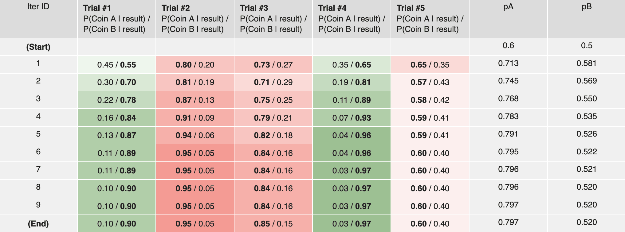
Our final estimation for $p_A, p_B$ is

$\hat p_A=0.797\\ \hat p_B=0.520$

Note that this result matches our intuition: Comparing to our result in the warm-up scenario, due to the uncertainty in coin identity, our final estimation for coin A is slightly lower than 0.8 (as “pulled down” by coin B), and our estimation for coin B is slightly higher than 0.45 (as “pulled up” by coin A).

To summarize, in order to infer $p_A, p_B$ from incomplete data with unknown coin identity at each trial, we follow the Expectation-Maximization (EM) algorithm as described below:

💡 Algorithm 2: Expectation-Maximization (EM) — Infer $p_A$ and $p_B$ from incomplete data.

• Repeat until converge:
  • E-Step: Compute the probability of each trial being coin A or coin B;
  • M-Step: Compute $\hat p_A, \hat p_B$ as normalized soft count.

Discussion

The intuition makes sense, but why is this method mathematically correct?

That is a very good question. In fact, it is worth noting that the “soft count” approach is an oversimplified version of the M-step that happens to be mathematically correct for this particular example (and the following GMM example). The general idea is that we can prove the likelihood function is monotonically non-decreasing after each iteration of E-step and M-step, so that our estimation for $p_A, p_B$ (or the “parameters”) gradually becomes better in the sense that it makes the observed coin tosses (or the “observation”) more likely to happen. I’m leaving the proof to the next post — check it out if you are interested! (warning: math ahead)

Does EM always converge to the global optimum?

It is not gauranteed that we will always arrive at the global optimum — quoting the Stanford CS229 course notes on the EM Algorithm, “Even for mixture of Gaussians, the EM algorithm can either converge to a global optimum or get stuck, depending on the properties of the training data.” That being said, in practice EM is considered to be a useful algorithm, as “Empirically, for real-world data, often EM can converge to a solution with relatively high likelihood (if not the optimum), and the theory behind it is still largely not understood.”

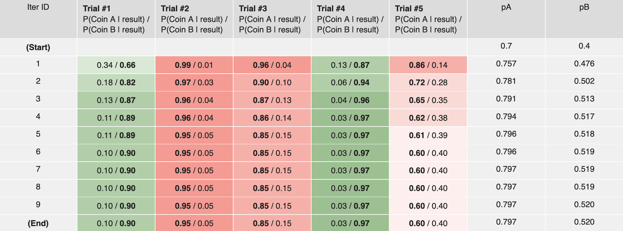
Do we get different results if we started at a different initial guess?

It is possible (though not gauranteed) that we still get the same result even if we started at a different initial guess. For instance, in the two coins example, a different guess $p_A^{(0)}=0.7, p_B^{(0)}=0.4$ produces the same results:

If we plot the likelihood function $\mathcal{L}(p_A, p_B) = \sum_{j=1}^5 \log\left[\sum_{p\in \{p_A, p_B\}}\dfrac{1}{2}C_{10}^{H_j}p^{H_j}(1-p)^{10-H_j}\right]$ (where $H_j$ is the number of head tosses in trial $j$) along with the intermediate results, it would become clear that both cases converge to the same optima through different optimization paths:

$p_A^{(0)}=0.6, p_B^{(0)}=0.5$	$p_A^{(0)}=0.7, p_B^{(0)}=0.4$

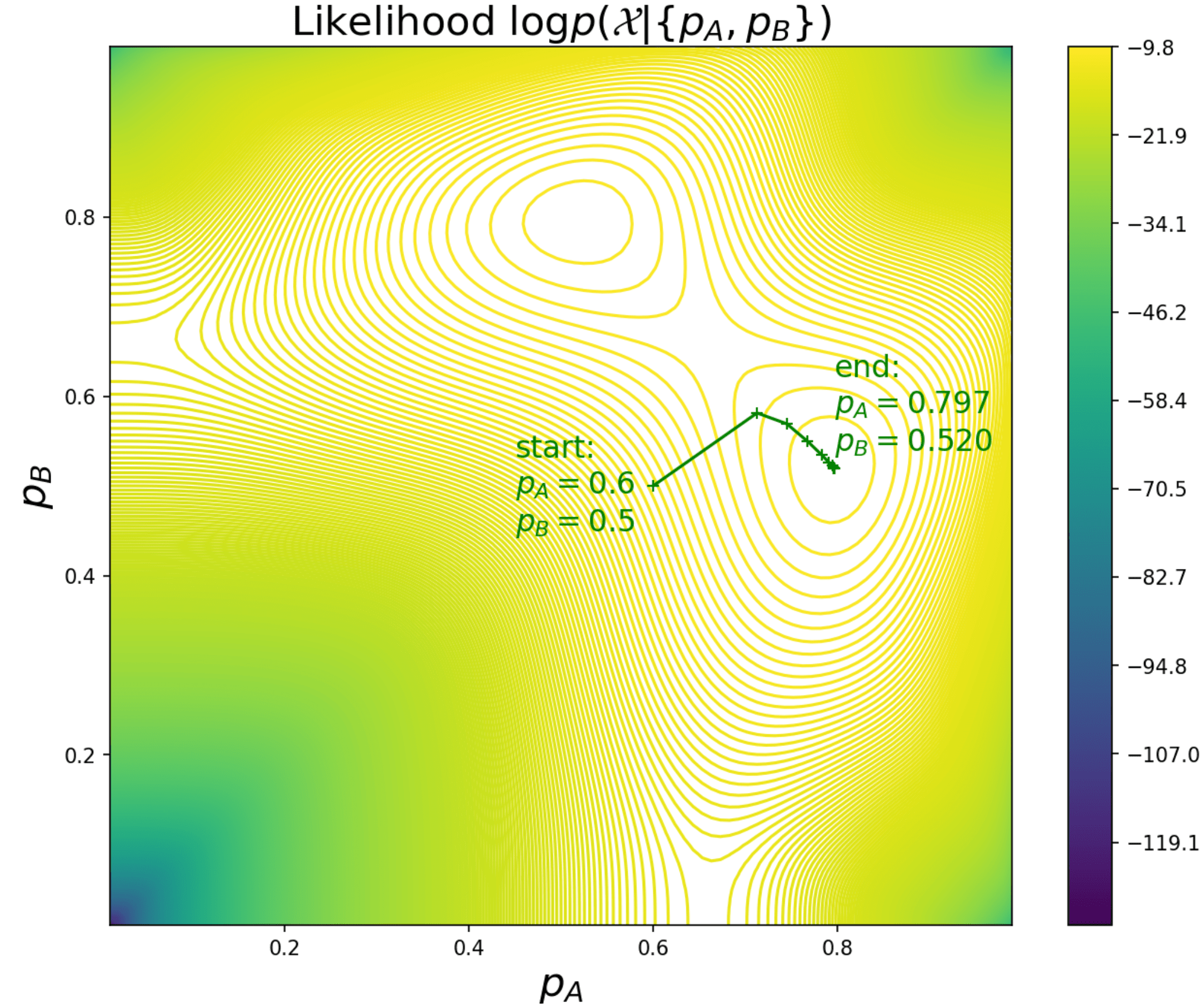
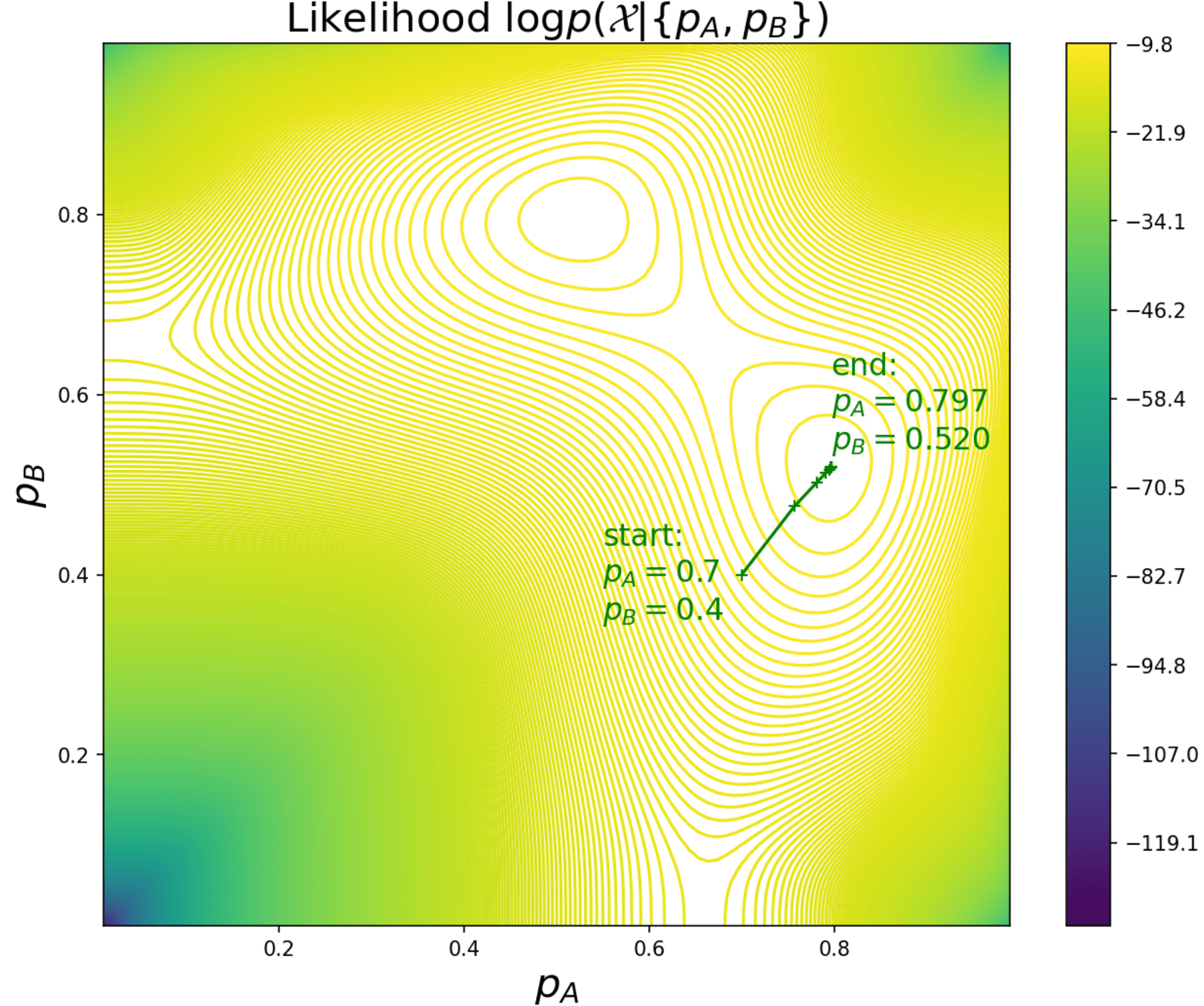
GMM example: Girls and boys

Now consider a new situation: Given 6 students whose heights are taken down in the following table, we’d like to infer the gender for each student (Note: in real life, inferring one’s gender based on their height might be a bad idea. This example is for educational purposes only).

Student ID	Gender	Height (cm)
#1	Unknown	168
#2	Unknown	180
#3	Unknown	170
#4	Unknown	172
#5	Unknown	178
#6	Unknown	176

For simplicity, we assume that the heights of the boys and the girls conform to normal distribution $\mathcal{N}(\mu_B, \sigma_B)$ and $\mathcal{N}(\mu_G, \sigma_G)$, respectively. Since the total distribution is the combination of two Gaussian distributions, this is called a Gaussian mixture model (GMM).

The problem is similar to the two coins: In order to infer the gender of each student, we need to know the parameter $\theta=\{\mu_B, \mu_G, \sigma_B, \sigma_G\}$; However, in order to estimate the parameter $\theta$, we need to know the gender of each student. Let’s see how the EM algorithm works in this scenario.

E-Step

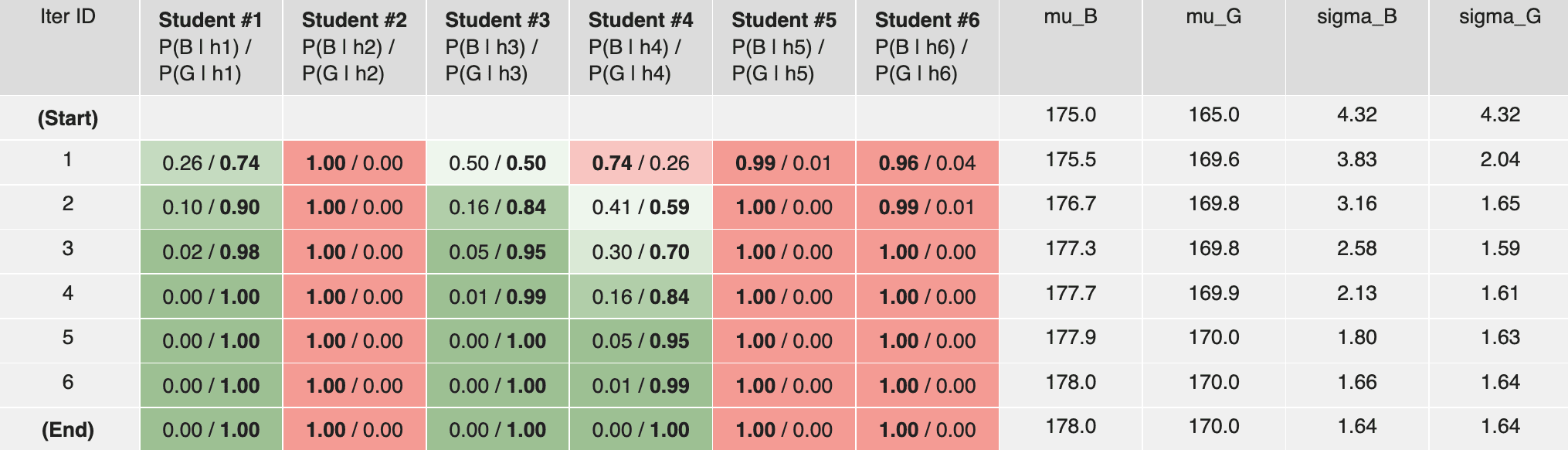
Remember that the key idea of the E-step is to infer how likely it is that a certain data point (i.e. a student) belongs to a certain category (i.e. boy or girl). Remember also that we need an initial guess for the parameter $\theta$ to kick start the computation, e.g. we may guess that the average height $\mu_B^{(0)}=175$ for boys and $\mu_G^{(0)}=165$ for girls, and the standard deviations $\sigma_B^{(0)}= \sigma_G^{(0)}=4.32$ (which is the standard deviation of the heights of all students). Under this setup, the probability of student #1 being a boy or a girl can be computed as:

$\begin{aligned} P(\text{boy} | \text{height=168cm}) &\propto P(\text{boy}, \text{height=168cm}) =\dfrac{1}{2}\cdot \mathcal{N}(x=168;~\mu=175, \sigma=4.32) \approx 0.012\\ P(\text{girl} | \text{height=168cm}) &\propto P(\text{girl}, \text{height=168cm}) = \dfrac{1}{2}\cdot \mathcal{N}(x=168;~\mu=165, \sigma=4.32) \approx 0.036\\\\ \therefore P(\text{boy} | \text{height=168cm}) &= \dfrac{0.012}{0.012+0.036}\approx0.26\\ P(\text{girl} | \text{height=168cm}) &= \dfrac{0.012}{0.012+0.036}\approx0.74 \end{aligned}$

Doing so for all 6 students gives us:

	Student #1	Student #2	Student #3	Student #4	Student #5	Student #6
P(boy | height)	0.26	1.00	0.50	0.74	0.99	0.96
P(girl | height)	0.74	0.00	0.50	0.26	0.01	0.04

M-Step

Remember that the key idea of the M-step is to estimate the parameters by counting each data point partially for each category. Similar to the two coins example, we modify the equation for mean and standard deviation by weighting using the probability from the E-step:

$\begin{aligned} \mu_B^{(1)} &= \dfrac{\textcolor{darkred}{0.26}\times168+\textcolor{darkred}{1.00}\times180+...+\textcolor{darkred}{0.96}\times176}{\textcolor{darkred}{0.26+1.00+...+0.96}} \approx 175.5\\\\ \mu_G^{(1)} &= \dfrac{\textcolor{green}{0.74}\times168+\textcolor{green}{0.00}\times180+...+\textcolor{green}{0.04}\times176}{\textcolor{green}{0.74+0.00+...+0.04}} \approx 169.6\\\\ {\sigma_B^{(1)}}^2 &= \dfrac{\textcolor{darkred}{0.26}\times(168-175.5)^2+...+\textcolor{darkred}{0.96}\times(176-175.5)^2}{\textcolor{darkred}{0.26+1.00+...+0.96}}\approx 3.83\\\\ {\sigma_G^{(1)}}^2 &= \dfrac{\textcolor{green}{0.74}\times(168-169.6)^2+...+\textcolor{green}{0.04}\times(176-169.6)^2}{\textcolor{green}{0.74+0.00+...+0.04}}\approx 2.04 \end{aligned}$

Repeating the E-step and the M-step for several iterations until convergence, we get the final answer: student #1, #3, #4 are most likely girls, while student #2, #5, #6 are most likely boys. We can also verify that the final values of $\mu_B, \mu_G$ are equal to the average heights of the male and the female students, respectively:

Why EM works | Log-Likelihood and ELBO

Now let’s dive into the math and answer the following questions — Why EM works? What is a more generalized form of the EM algorithm that can be applied to problems other than two coins and GMM?

Log-Likelihood

To begin with, given a dataset with $n$ data points and unknown parameter $\theta$, the core problem that EM attempts to solve is to maximize the log-likelihood of the observed data:

$\theta^* = \arg\max_\theta\sum_{i=1}^n \log P(x^{(i)}; \theta)$

For instance, in the two coins example, the observation $x^{(i)}$ is the coin tossing result at the $i$-th trial, and the parameter $\theta=\{p_A, p_B\}$; In the GMM example, the observation $x^{(i)}$ is the height of the $i$-th student, and the parameter $\theta=\{\mu_B,\mu_G,\sigma_B,\sigma_G\}$.

Hidden Variable

Remember that in both examples, there’s missing information in the data, usually called a “hidden” variable, denoted as $z^{(i)}$. For instance, in the two coins example, the hidden variable $z^{(i)}$ is the coin identity at the $i$-th trial; In the GMM example, $z^{(i)}$ is the gender of the $i$-th student.

In order to compute the likelihood function, a common practice is to “break down” the likelihood into all categories by marginalizing over the hidden variable $z^{(i)}$:

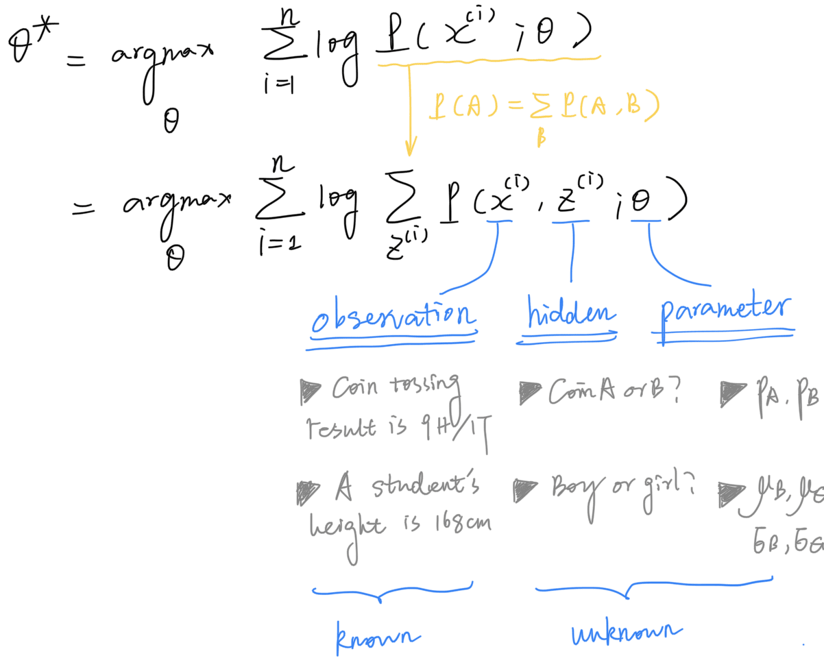
For the sake of simplicity, we will consider the optimization for a single example $x$ first, drop the outer sum and the superscript $^{(i)}$, and add them back after we derived the algorithm. Our optimizaton target becomes:

$f(\theta) = \log\sum_zP(x, z;\theta)$

Note that we get a expression in the “log of sum” format. Quoting UMich EECS 545 lecture notes, in general this likelihood is non-convex with many local minima and hard to optimize:

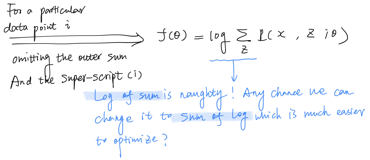
ELBO (Evidence Lower Bound)

The good news is that we can construct a lower bound function $g(\theta)$ (usually called the ELBO, Evidence Lower Bound) — in the much nicer “sum of log” format, and use it as a proxy to optimize the log-likelihood function $f(\theta)$.

In order to construct such a lower bound, one important, yet unintuitve trick is to introduce a new variable $\textcolor{darkblue}{q(z)}$ into the objective function, as it allows us to swap the order between log and sum. $q(z)$ is an arbitrary probability distribution over $z$ that satisfies $\sum_zq(z)=1$. To put it into context, this is the probability distribution that we computed in the E-step, e.g. the probability that a certain trial belongs to coin A or B, or the probability that a certain student is male or female. We will later see that it should converge to the posterior distribution $P(z|x; \theta^*)$ as the algorithm iterates and converges to the optimal paramter $\theta^*$:

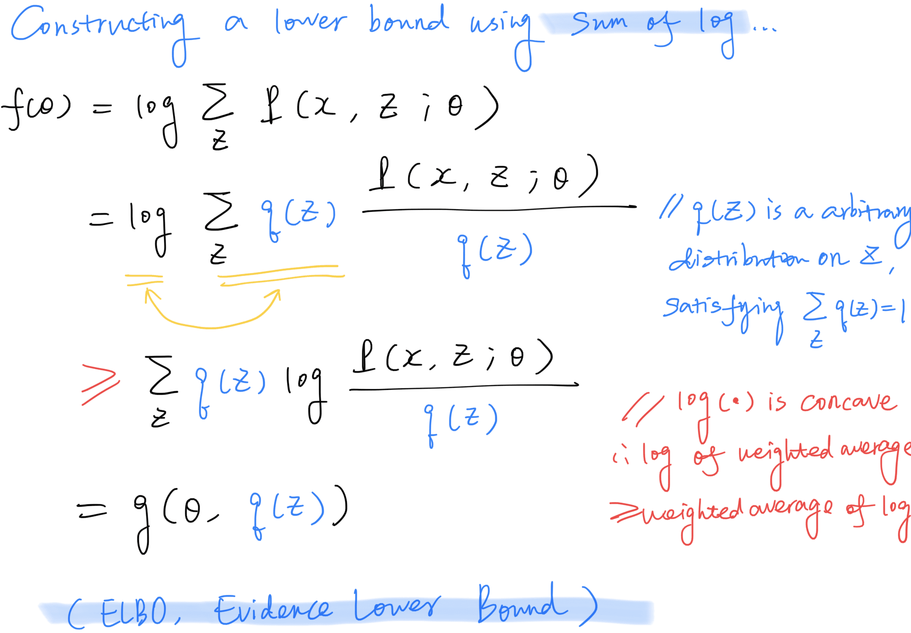
Note that it is possible for the inequality to become an equality: If we set $\textcolor{darkblue}{q(z)}=P(z|x; \theta)$, the argument to $\log(\cdot)$ becomes $P(x;\theta)$, which is a constant value with respect to $z$ — for which it does not matter whether the weighted average or the logarithm is applied first. Therefore, in that case the equality is satisified, and the ELBO $g$ becomes a tight lower bound for the log-likelihood $f$.

Iterative Optimization

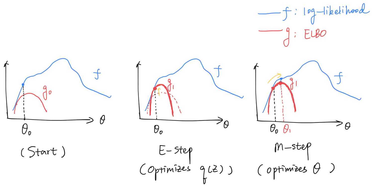
But how can we optimize $f$ using its lower bound $g$? The answer is that we can do it in an iterative fashion (see the figure below):

1. In the E-step, we “lift” the shape of $g$ such that it reaches $f$ at the current $\theta$. This is achievable by setting $q(z)=P(z|x;\theta)$, as mentioned above;
2. In the M-step, we find a new $\theta$ that maximizes $g$, such that we arrive at a better solution than the beginning of this iteration.

Convergence

Formally, it can be proved that the log likelihood function $f$ is monotonically non-decreasing across the iterations:

$f(\theta_{t+1}) \underbrace{\geq}_{\text{Log-likelihood }\geq \text{ ELBO}} g(\theta_{t+1}, q_t) \underbrace{\geq}_{\text{M-step}} g(\theta_{t}, q_t)\underbrace{=}_{\text{E-step}}f(\theta_t)$

This also proves that the EM algorithm will eventually converge (though the result is not guaranteed to be the global optimum).

In order to visualize the convergence process, I constructed an example with the two coins problem: Suppose we keep $p_A=0.797$ (which is already the optimal value) fixed and use EM to optimize $p_B$ (initialized to $p_B^{(0)}=0.2$), here is what we get in 3 EM iterations (Note how the ELBO is “lifted” in the E-step and maximized in the M-step):

Simplifying the M-step

Now if you are convinced that the EM algorithm will eventually converge to a point better than the initial guess, let’s move on to the actual computation part.

Remember that in the M-step, we need to find the maximizer for the ELBO function, which looks quite complex:

$g(\theta, ~\textcolor{darkblue}{q(z)}) = \sum_z q(z) \log \dfrac{P(x, z; \theta)}{q(z)}$

It turns out that we can simplify this equation by expanding it and removing an irrelevant term:

$\begin{aligned} &~~~~~\arg\max_\theta \sum_z q(z) \log \dfrac{P(x, z; \theta)}{q(z)}\\ &= \arg\max_\theta \sum_z q(z) \left[\log P(x, z; \theta) - \log q(z)\right]\\ &= \arg\max_\theta [\sum_z q(z) \log P(x, z; \theta) \underbrace{-\sum_z q(z)\log q(z)}_{\text{constant wrt } \theta \atop \text{can be ignored}}]\\ &=\arg\max_\theta\sum_z q(z) \log P(x, z; \theta)\\ &= \arg\max_\theta \displaystyle \mathop{\mathbb{E}}_{z\sim q(z)}\log P(x, z; \theta) \end{aligned}$

To put it into words, this basically says “find the $\theta$ that works the best in the average scenario”, where the “average” is weighted by a distribution $q(z)$ — calculated in the E-step — that tells how likely it is that this particular data point $x$ (e.g. a coin tossing trial) belongs to a certain category $z$ (e.g. coin A or B) given the observation.

Adding back the sum over all data points $i=1…n$, our final formula for the M-step becomes:

$\theta_{t+1}=\arg\max_\theta \sum_{i=1}^n \displaystyle \mathop{\mathbb{E}}_{z^{(i)}\sim q^{(i)}(z^{(i)})}\log P(x^{(i)}, z^{(i)};~ \theta)$

To summarize, a more generalized version of the EM algorithm looks like:

💡 Algorithm 3: Expectation-Maximization (EM) — Final version

• Input: Observation $\{x^{(1)}…x^{(n)}\}$, initial guess for the parameter $\theta_0$
• Output: Optimal parameter value $\theta^*$ that maximizes the log-likelihood

  $\mathcal{L}(\theta)=\sum_{i=1}^n \log P(x^{(i)};\theta)$

• For $t=1…T$ (until converge):
  • E-Step: For each $i=1…n$, compute the hidden posterior:

    $q^{(i)}(z^{(i)})=P(z^{(i)}|x^{(i)};\theta_t)$

  • M-Step: Compute the maximizer for the evidence lower bound (ELBO):

    $\theta_{t+1}=\arg\max_\theta \sum_{i=1}^n \displaystyle \mathop{\mathbb{E}}_{z^{(i)}\sim q^{(i)}(z^{(i)})}\log P(x^{(i)}, z^{(i)};~ \theta)$

Now you may wonder: How can the two coins example and the GMM example fit into this framework? The final form seems so complicated! In the next post, we will provide proofs that our previous methods used in these two examples are mathematically equivalent to Algorithm 3. You will probably be surprised that such simple and intuitive algorithms take so much to prove their correctness!

References

[1] What is the expectation maximization algorithm? Chuong B Do, Serafim Batzoglou. Nature, 2008. [paper]

[2] Expectation Maximization. Benjamin Bray. UMich EECS 545: Machine Learning course notes, 2016. [course notes]

[3] The EM algorithm. Tengyu Ma, Andrew Ng. Stanford CS 229: Machine Learning course notes, 2019. [course notes]

[4] Bayesian networks: EM algorithm. Stanford CS 221: Artificial Intelligence: Principles and Techniques slides, 2021. [slides]

[5] 如何感性地理解EM算法？工程师milter. 简书, 2017. [blog post]

[6] Coin Flipping and EM. Karl Rosaen, chansoo. UMich EECS 545: Machine Learning Materials. [Jupyter Notebook]