Understanding the VAE Model

I believe most beginners to VAE (variational autoencoder) will encounter the following two types of introductions when searching for tutorials online, and may inevitably get a bit disoriented when they find the logical connections not very intuitive:

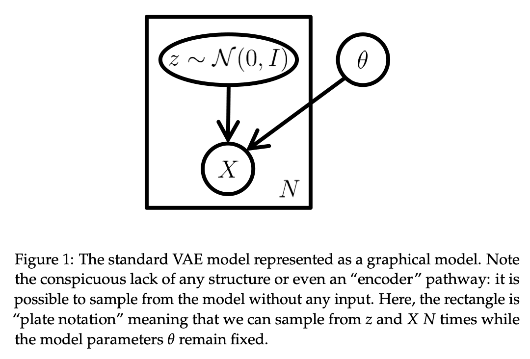
• From a theoretical perspective, the VAE is a generative model that learns a probability distribution $P(x)$ for datapoints that can be directly sampled from. It assumes that each of the datapoint $x$ is generated according to the following process: (1) A latent variable $z$ is sampled from a predefined prior distribution $P(z)$, and then (2) A datapoint $x$ is sampled from the conditional distribution $P(x|z)$ (usually a neural network parametrized by learnable parameters $\theta$). The end goal is to maximize the dataset likelihood function $\sum \log P(x)$.

The graphical model of VAE. Image credit: [1]

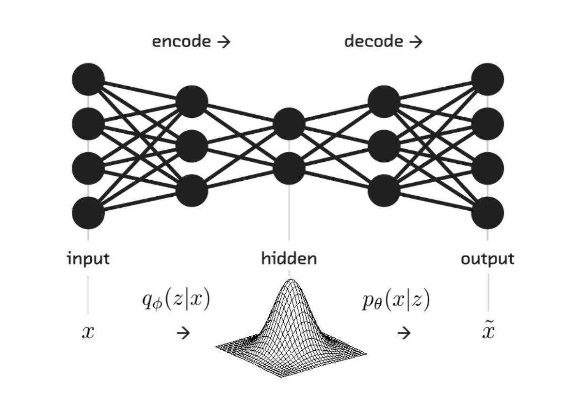
• From a technical perspective, the VAE uses an encoder network to map each datapoint $x$ to a distribution of its latent variable $z$, and then uses a decoder network to map it back to a distribution of its reconstruction $\hat x$. The optimization goals are to (1) make $\hat x$ as close to $x$ as possible, and to (2) learn a meaningful latent space for $z$, such that we can generate novel samples by decoding from random noise.

The encoder-decoder architecture of VAE. Image credit: The Fast Forward Labs blog

This article aims to explain the math behind VAE and thereby clarify that the above two perspectives are in fact (almost) equivalent to each other. The codes for all the examples mentioned in this article can be found at https://github.com/mistylight/Understanding_the_VAE_Model.

📚 NOTE: This article assumes that the reader is familiar with the Expectation-Maximization (EM) algorithm. In case you are unfamiliar with EM, I have another tutorial on this topic: Understanding the EM Algorithm.

Problem Statement

Given a dataset $\mathcal{X} = \{x^{(1)}, x^{(2)}, ..., x^{(n)}\}$, we assume that each of the datapoint $x^{(i)}$ is generated by first sampling a latent variable $z^{(i)}$ from a known prior distribution $P(z)$, and then sampling $x^{(i)}$ from a conditonal distribution $P(x|z^{(i)};\theta)$ parametrized by $\theta$. The ultimate goal is to find the optimal value of $\theta$ that maximizes the dataset likelihood:

$\theta_{\max} = \arg\max_\theta \sum_{i=1}^n \log P(x^{(i)}; \theta)$

Take the MNIST dataset as an example, one may think of $x^{(i)}$ as an image containing one hand-written digit, and imagine $z^{(i)}$ as a latent vector indicating the represented digit itself plus some style options such as the font family, font size, font weight, etc.

In image generation, a common choice of $z$ is the standard normal distribution $\mathcal{N}(0, 1)$, and usually $P(x|z^{(i)};\theta)$ is modeled as a neural network with learnable parameter $\theta$ (e.g. A Bernoulli distribution with probability $f(z;\theta)$, where $f$ is a neural network taking $z$ as an input and parametrized by $\theta$).

One may wonder why it is valid to assume $P(z)$ to be Gaussian. This is because it is provable that “any distribution in d dimensions can be generated by taking a set of d variables that are normally distributed and mapping them through a sufficiently complicated function” (cited from page 6 of [1]). Therefore, as long as $P(x|z;\theta)$ is a sufficiently powerful function approximator, e.g. a high-capacity neural network, then the resulting distribution of $x$ can still be arbitrarily complex, which means the approximation error introduced by the assumption on $P(z)$ is reasonably small.

The Challenge with EM

Now that we are presented with a max-likelihood problem with both unknown hidden variables and parameters, one may think of the EM algorithm as it is one of the most commonly used methods for solving problems of this kind.

💡 Algorithm 1: Expectation-Maximization (EM)

• Input: Observation $\{x^{(1)}…x^{(n)}\}$, initial guess for the parameter $\theta_0$
• Output: Optimal parameter value $\theta^*$ that maximizes the log-likelihood

  $\mathcal{L}(\theta)=\sum_{i=1}^n \log P(x^{(i)};\theta)$

• For $t=1…T$ (until converge):
  • E-Step: For each $i=1…n$, compute the hidden posterior:

    $Q^{(i)}(z^{(i)})=\textcolor{red}{\underbrace{P(z^{(i)}|x^{(i)};\theta_t)}_{\text{intractable}}}$

  • M-Step: Compute the maximizer for the evidence lower bound (ELBO):

    $\theta_{t+1}=\arg\max_\theta \sum_{i=1}^n \displaystyle \mathop{\mathbb{E}}_{z^{(i)}\sim Q^{(i)}(z^{(i)})}\dfrac{\log P(x^{(i)}, z^{(i)};~ \theta)}{Q^{(i)}(z)}$

Unfortunately, recall that the E-step of the EM algorithm requires that we compute the posterior distribution $P(z|x;\theta)$, which is usually intractable if $z$ is a continuous variable and the conditional distribution $P(x|z;\theta)$ is defined as a neural network. This is because in order to compute the posterior, one needs to compute the integral over all possible values of $z$, which is intractable in practice (dropping the $\theta$ for simplicity):

$P(z|x) = \dfrac{P(x|z)P(z)}{P(x)} = \dfrac{P(x|z)P(z)}{\int_z P(x|z)P(z) dz}$

Variational Posterior

Now that the problem is the intractability of computing $P(z|x;\theta)$ in the E-step, what if we borrow the idea from variational inference – introduce an approximate posterior $Q(z|x;\phi)$ which is tractable to compute, skip the E-step, and directly plug it into the M-step, where $P$ and $Q$ are optimized altogether?

Modified EM: Use gradient descent to optimize ELBO w.r.t. both $P$ and $Q$:

$\theta^*, \phi^* = \arg\max_{\theta, \phi} \sum_{i=1}^n \displaystyle \mathop{\mathbb{E}}_{z^{(i)}\sim Q(z|x^{(i)};\phi)}\dfrac{\log P(x^{(i)}, z^{(i)};~ \theta)}{Q(z^{(i)}|x^{(i)};\phi)} \quad (*)$

In practice, a common choice of $Q(z|x;\phi)$ is a Gaussian distribution $\mathcal{N}(\mu(x;\phi), \sigma(x;\phi))$, where $\mu, \sigma$ are neural networks taking $x$ as an input and parametrized by $\phi$. It has several nice properties, such as the ease of computation, which we will see later on.

The $Q(z|x;\phi)$ network is also frequently called the “encoder” as it maps each datapoint $x$ to a distribution of its corresponding latent variable $z$; The $P(x|z;\phi)$ network is commonly referred to as the “decoder” as it maps a given latent variable $z$ to a distribution of reconstructed datapoint $\hat x$.

The encoder-decoder architecture of VAE. Image credit: The Fast Forward Labs blog

Note that the main difference between (*) and the original EM algorithm is that: In the original EM algorithm, $Q(z^{(i)}|x^{(i)}) := P(z^{(i)}|x^{(i)};\theta)$ was precomputed in the E-step for every single datapoint in order to align the ELBO with the likelihood; In contrast, in the modified EM algorithm (*) $Q(z|x;\phi)$ is a neural network taking $x^{(i)}$ as input, producing $Q(z^{(i)}|x^{(i)};\phi)$ as output, and jointly learned along with $P$. It is worth noticing that in this case, the optimization objective shifts from the dataset likelihood to the ELBO (Evidence Lower Bound), because we no longer get the correction from the E-step. This is an approximation to make the computation tractable.

An example EM optimization process, note how the ELBO is "aligned" with the likelihood at the current value of θ in the E-step. This ensures that we are essentially optimizing the dataset likelihood instead of ELBO. In contrast, if we omit the E-step as discussed in this section, the optimization objective shifts from the likelihood to the ELBO. We’ll quantify this error in the next section.

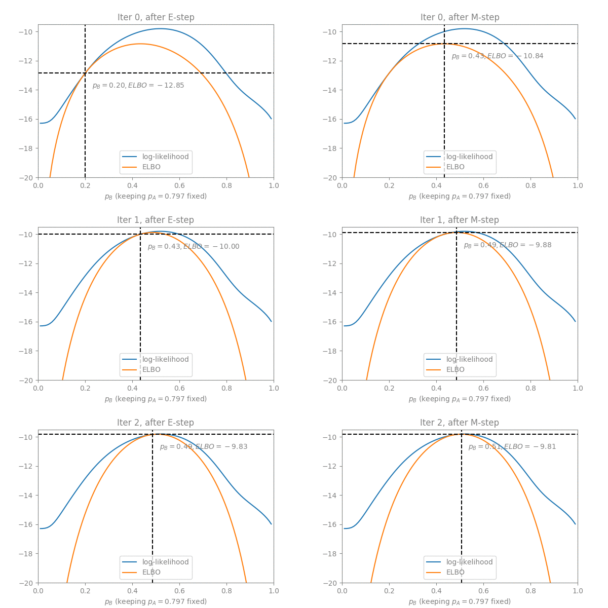
The question here is: How much error are we introducing by omitting the E-step?

Quantifying the Approximation Error

To begin with, there are two types of errors when we optimize for a machine learning problem (see the Stanford CS221 course note for a more in-depth introduction):

• Approximation error: Errors stemming from the gap between the model family and the true distribution. In the case of VAE, this gap is caused by the omission of the E-step – the optimization objective has changed from the dataset likelihood (true objective) to ELBO (optimization proxy)!
• Estimation error: Errors caused by the inability to find the best model within the model family. In the case of VAE, this means the gap between the final ELBO and the optimal ELBO, and it usually stems from the imperfection of the stochastic gradient descent algorithm.

Approximation error v.s. Estimation error. Figure credit: Stanford CS221 course note

We are mostly interested in the approximation error – what is the best possible model we can get in this scenario?

Recall the definition of ELBO for a single datapoint $x$ and its corresponding latent variable $z$ (here, we are dropping the superscriptions and $\theta, \phi$ for clarity), which was optimized in the M-step of EM:

$\text{ELBO}(P, Q) = \int_z Q(z|x) \log \dfrac{P(x, z)}{Q(z|x)}dz = \mathbb{E}_{z\sim Q(z|x)}[\log \dfrac{P(x, z)}{Q(z|x)}]$

It is called the “evidence lower bound”, mainly because it is provable that it is a lower bound for the dataset likelihood, which is the true objective we wish to optimize:

$\text{ELBO}(P, Q)\leq\log P(x)$

The equality is satisfied if and only if $Q(z|x) \equiv P(z|x)$. Further, we can prove that the gap between ELBO and the dataset likelihood is exactly the KL divergence between the approximate posterior and the true posterior. Intuitively, this is exactly the error we introduced by omitting the E-step:

$\begin{aligned} &\quad\text{ELBO}(P, Q) \\ &= \underline{\mathbb{E}_{z\sim Q(z|x)}[\log \dfrac{P(x, z)}{Q(z|x)}]} \\ &= \underline{\mathbb{E}_{z\sim Q(z|x)}[\log P(x, z) ]} - \mathbb{E}_{z\sim Q(z|x)}[\log Q(z|x) ] \\&= \underline{\mathbb{E}_{z\sim Q(z|x)}[\log P(x) ]} + \mathbb{E}_{z\sim Q(z|x)}[\log P(z|x) ] - \mathbb{E}_{z\sim Q(z|x)}[\log Q(z|x) ] \\&= \log P(x) + \underline{\mathbb{E}_{z\sim Q(z|x)}[\log P(z|x) ] - \mathbb{E}_{z\sim Q(z|x)}[\log Q(z|x) ]} \\&= \log P(x) - \underline{\mathbb{E}_{z\sim Q(z|x)}[\log\dfrac{Q(z|x)}{P(z|x)}]} \\&= \log P(x) - \underbrace{\text{KL}[Q(z|x)\| P(z|x)]}_{\text{gap between ELBO and likelihood}} \end{aligned}$

It turns out maximizing the ELBO is equivalent to maximizing the likelihood while minimizing the gap between the approximation posterior and the true posterior. It though remains questionable how much error is introduced by the last KL term as it deviates the optimization from the true likelihood. This deviation reflects the tradeoff between the accuracy v.s. tractability: At one extreme lies the EM algorithm, where the KL term is zeroed by setting $Q(z|x) \equiv P(z|x)$ at the cost of intractable integral computation; At the other extreme, if $Q(z|x)$ is defined as a very low-capacity distribution that approximates $P(z|x)$ very poorly, then the KL term becomes unignorable and the optimization objective will be completely off from the true likelihood.

Quoting [1], we can have zero approximation error only if there exists a certain pair of $(\theta, \phi)$ that maximizes $\log P(x)$ AND satisfies $P(z|x)$ being Gaussian for all $x^{(i)}$s. Does this optimal solution always exist? To the best of my knowledge, as of 2022, we cannot answer this question super well. There is though a body of research investigating the approximation error introduced by the KL term, either empirically or theoretically. For instance, [5] shows when both encoder and decoder are exponential families, the KL term can pull the models from the likelihood optimizers to a subset allowing the KL term to be zero, which can be detrimental to the performance if this subset is too restricted. [6] studies how is error influenced by various design choices, such as the capacity of the encoder network. In my view, [1] summarizes the status of this line of research quite well: “future theoretical work may show us how much approximation error VAEs have in more practical setups.”

Implementing the Optimization

As of this point, we’ve established that the VAE is kind of like a modified version of EM that compromises accuracy for tractability, and that as a result, it optimizes the ELBO which is similar to the dataset likelihood but not exactly the same. Let’s now focus on how to actually perform the optimization. The process involves some math tricks, but the ELBO eventually breaks down to two tractable objectives which are feasible to optimize with stochastic gradient descent:

$\begin{aligned} &\quad\text{ELBO}(P, Q) \\ &= \underline{\mathbb{E}_{z\sim Q(z|x)}[\log \dfrac{P(x, z)}{Q(z|x)}]} \\ &= \underline{\mathbb{E}_{z\sim Q(z|x)}[\log P(x, z) ]} - \mathbb{E}_{z\sim Q(z|x)}[\log Q(z|x) ] \\&= \mathbb{E}_{z\sim Q(z|x)}[\log P(x|z) ] + \underline{\mathbb{E}_{z\sim Q(z|x)}[\log P(z) ] - \mathbb{E}_{z\sim Q(z|x)}[\log Q(z|x) ]} \\&= \mathbb{E}_{z\sim Q(z|x)}[\log P(x|z) ] -\underline{\mathbb{E}_{z\sim Q(z|x)} [\dfrac{Q(z|x)}{P(z)}]} \\&= \underbrace{\mathbb{E}_{z\sim Q(z|x)}[\log P(x|z) ]}_{\text{reconstruction}} - \underbrace{\text{KL}[Q(z|x) \| P(z)]}_{\text{latent space regularization}} \end{aligned}$

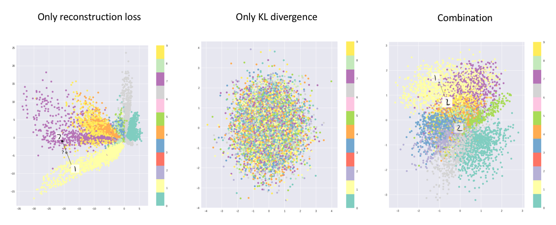
Intuitively, the first term encourages the reconstruction of the training set datapoints, for it maximizes the likelihood of training set datapoint $x$ when the latent variable $z$ is sampled from the encoder. This encourages the train set datapoints to be resampled from the decoder during training, therefore it’s usually referred to as the “reconstruction loss”; The second term regularizes the structure of the latent space of $z$, for it encourages the distribution of $z$ values visited during training (produced by the encoder) to be as close to our predefined prior of $z$ (usually $\mathcal{N}(0, 1)$) as possible. This is especially useful if we wish to generate new datapoints by first sampling $z$ from $\mathcal{N}(0, 1)$ and then sampling $x$ from the decoder, because if there exist some values of $z$ with high probability density in $\mathcal{N}(0, 1)$ (therefore making them very likely to be sampled) but rarely visited during training because the encoder assigns extremely low probability density to them, then it’d be very hard for the decoder to perform well on those unseen $z$ values.

The latent space of VAE with different loss functions. Image credit: Jeremy Jordan’s blog

Computing the Reconstruction Loss

In stochastic gradient descent, the reconstruction loss $\mathcal{L}_{\text{recon}} = \mathbb{E}_{z\sim Q(z|x)}[\log P(x|z) ]$ can be approximated by replacing the expectation operation with the batch mean as is the standard practice in deep learning:

$\mathcal{L_\text{recon}} \approx \dfrac{1}{B}\sum_{i=1}^B \log P(x^{(i)}|z^{(i)};\theta)$

Where, $B$ is the batch size, $x^{(i)}$ are datapoints from the train set, and $z^{(i)}$ are sampled from $Q(z|x^{(i)};\phi)$. The tricky part is that the gradient cannot back propagate through the sampling operation, therefore it’d be hard to compute the gradient with respect to $Q$, i.e. $\nabla_\phi \mathcal{L}_{\text{recon}}$. Fortunately, there is a math trick called “reparametrization” that solves this problem when $Q$ is defined as a Gaussian distribution $\mathcal{N}(\mu(x;\phi), \sigma(x;\phi))$: We can just sample $\epsilon^{(i)} \sim \mathcal{N}(0, 1)$ which is independent of $Q$ and then $z^{(i)} = \mu(x^{(i)}; \phi)\cdot \epsilon^{(i)} +\sigma(x^{(i)};\phi)$ would conform to exactly the same distribution as $Q$. This way we decouple the sampling procedure from the parameter optimization, and as a result we can now proceed with back propagation as normal:

$\mathcal{L_\text{recon}} \approx \dfrac{1}{B}\sum_{i=1}^B \log P(x^{(i)}\mid\mu(x^{(i)}; \phi)\cdot \epsilon^{(i)} +\sigma(x^{(i)};\phi);\theta)\\ \text{where } \epsilon^{(i)} \sim \mathcal{N}(0, 1)$

When the training set datapoints $x^{(i)}$s are binary (e.g. black and white images), then if $P(x|z;\theta)$ is defined as the Bernoulli distribution, then the reconstruction loss is equivalent to the binary cross entropy (BCE) loss; Otherwise if $P(x|z;\theta)$ is defined as the Gaussian distribution, then the reconstruction loss is equivalent to a weighted L2 loss.

Computing the KL Divergence Loss

When both $Q(z|x;\phi)$ and $P(z)$ are defined as a Gaussian distribution, The KL divergence loss $\mathcal{L}_{\text{KL}} = \text{KL}[Q(z|x) \| P(z)]$ can be straightforwardly computed as the KL divergence between two multivariate Gaussian distributions, which has a closed-form expression (the derivation can be found at this Stack Exchange thread):

$\mathcal{L}_{\text{KL}} = \dfrac{1}{B}\sum_{i=1}^B\dfrac{1}{2}[-\sum_{j=1}^D (2\log \sigma_j+1) +\sum_{j=1}^D\sigma_j^2+\sum_{j=1}^D\mu_j^2]$

Where, $B$ is the batch size, $D$ is the dimension of $z$. $i$ indexes over the train set datapoints, $j$ indexes over dimensions of $z$. $\sigma_j, \mu_j$ refer to the $j$-th dimension of the mean and the variance of $Q(z|x;\phi)$, respectively.

To summarize: The encoder network $Q(z|x;\phi)$ and the decoder network $P(x|z;\theta)$ can be optimized end-to-end with loss function $\mathcal{L} = \mathcal{L}_{\text{recon}}+\mathcal{L}_{\text{KL}}$ using stochastic gradient descent.

Example: MNIST

Now that we’ve clarified the structure and the optimization technique of VAE, let’s take a look at the tasks that VAE made possible. For this purpose, we’ll use the MNIST hand-written digit dataset and train a VAE network with CNN encoder and decoder architectures. My implementation can be found at https://github.com/mistylight/Understanding_the_VAE_Model.

Latent Space

If we map each datapoint $x$ to its corresponding latent variable $z$ with the encoder, and then project it to 2D with PCA, here is what we get:

A visualization of the latent space of VAE trained on MNIST, projected to 2-dimension with PCA.

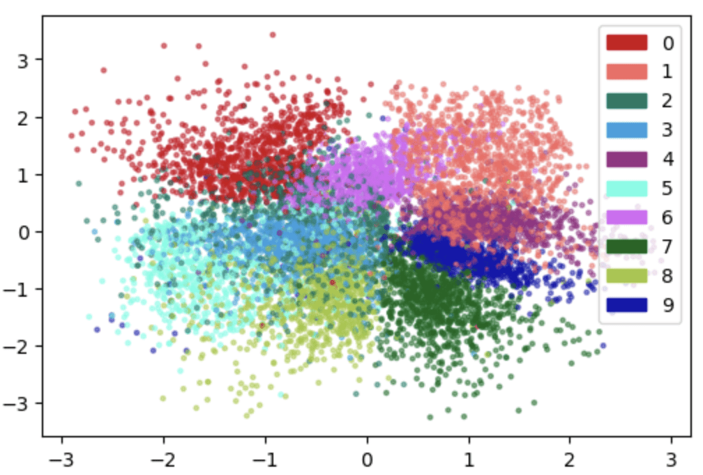
There are two noticeable features: First, latents for the same digit tend to cluster together, while latents for different digits tend to occupy different regions of the space; Second, the latent space regions occupied by different digits gather together compactly, leaving almost no gap in between. The first feature allows for retrieving images with the same digit as a reference image, and the second feature allows for sampling from the latent space and generating a new image accordingly (otherwise our sample may fall into a “hole” of the latent space which is unseen during training!). This indicates that the VAE learns a meaningful internal representation for the data, which is one of the main reasons for its popularity.

Reconstruction

One may wonder how much information is preserved during the “compression” from the high dimensional $x$ (a 28x28 image) to the low dimensional $z$ (a 10D vector in our experiment). This compression happens at the connection between encoder and decoder, which is commonly referred to as the “bottleneck”.

One way to look at this problem is to first map an input image $x$ to its corresponding $z$ with the encoder, and then map it back to a reconstructed image $\hat x$ with the decoder. Here we show some pairs of $(x, \hat x)$:

Input image x (left) and its corresponding VAE reconstruction x-hat (right).

Note how the VAE preserves the identity of the digit and (almost) keeps the angle of the input. However, the details might be a bit off, and most noticeably the edges are always blurry. This indicates that the most important information of the input image is preserved but the finer details are mostly lost. We will also discuss the issue of blurriness in the FAQ section.

Interpolation

Remember the latent space is compact with almost no gap between. Then what if we start off from one point in the latent space and gradually travel to another point? What will the points in-between look like if we decode them into images?

Interpolation between two points in the latent space.

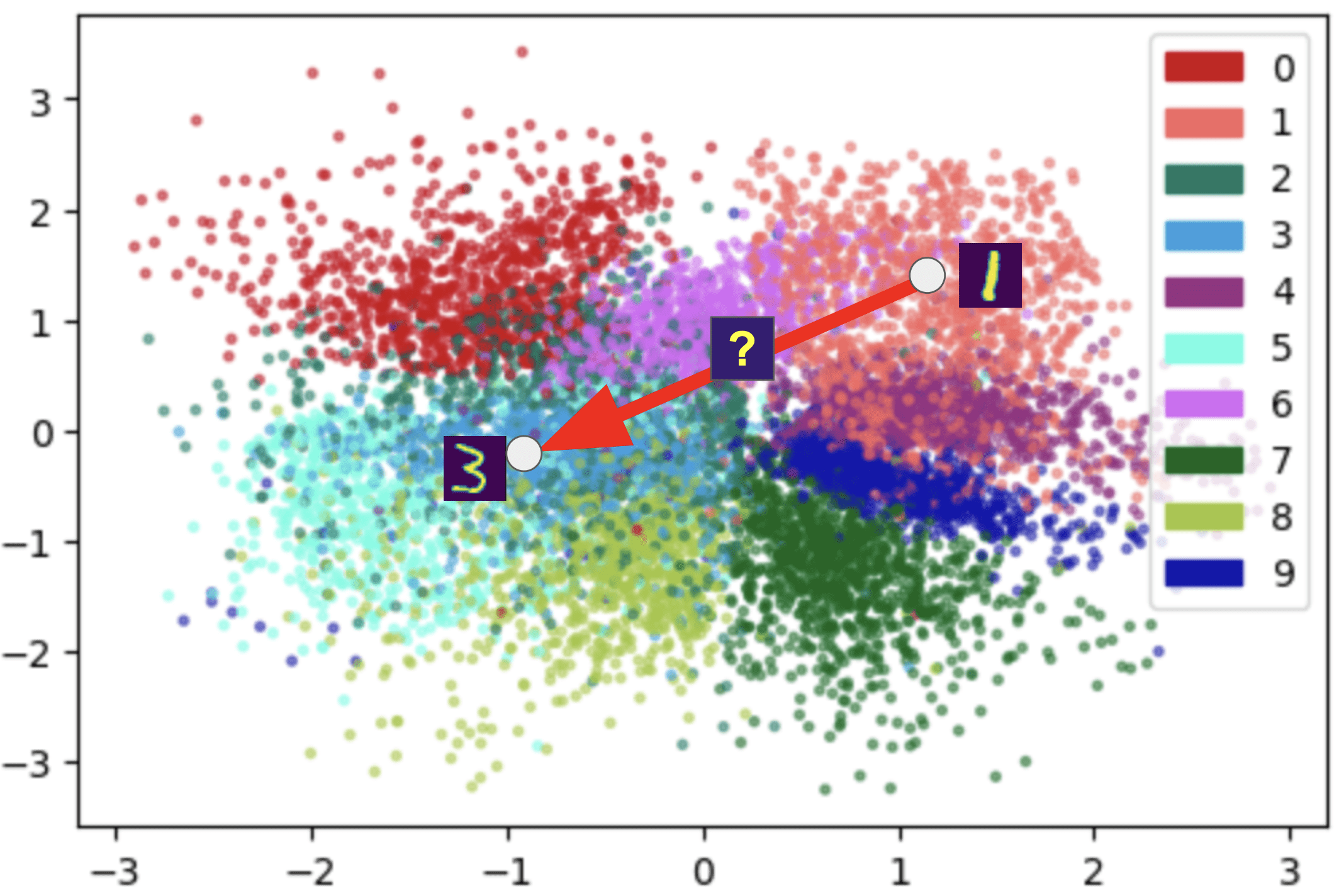
Here, we take two images $x_A, x_B$ from the test set of MNIST and sample 3 different points as the linear combination of their latent variables $z_A, z_B$, weighted by 25%, 50%, 75%, respectively. The results are as below:

The interpolation between two test images xA, xB. From left to right: xA, xA-hat, the 3 interpolations in between, xB-hat, xB.

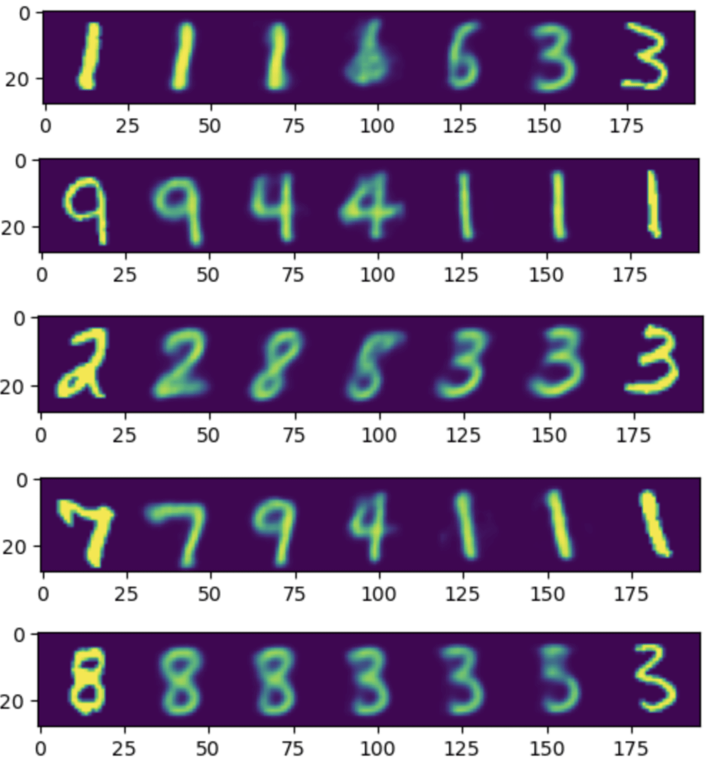
It is interesting to see how the shape of the first digit gradually deforms to that of the second one. Note that if the path between the two latent variables crosses the latent space of a new digit (as is the case with the 1 -> 3 interpolation in the first row, the path crosses the latent space of 6, as is shown in the latent space visualization), then we might see a new digit emerging during the interpolation. In practice, this interpolation may enable applications such as animation generation, which is very useful in the real world.

Sample and Generate

Wouldn’t it be cool if there was a button that randomly generates a brand new image every time you press it (as an ex-graphic designer, this has long been a dream of mine)? It turns out the VAE is capable of doing exactly this – you randomly sample a $z \sim \mathcal{N}(0, 1)$, use the decoder to map it to image, and that’s it! Here are some samples of the generated image:

Novel hand-written digit images generated by VAE.

FAQ

VAE vs AE?

Before the invention of VAE, there is another family of models called the autoencoder (AE). The major difference between them is that the AE only optimizes for the reconstruction loss and doesn’t have the KL divergence loss to regularize the latent space. As a result, the AE doesn’t have the generative power of VAE, because when randomly sampling a latent variable from $\mathcal{N}(0, 1)$, there’s a great chance of falling into a “hole” unseen during training, resulting in poor decoding results. The “Visualization of latent space” of Jeremy Jordan’s blog has an excellent explanation for this.

VAE vs GAN?

In recent years, generative adversarial networks (GANs) have been increasingly popular and achieve the state-of-the-art performance in most image generation tasks. The images generated by GAN are usually much more plausible, because the GAN uses a higher-level loss function produced by a deep network (the discriminator) instead of the low-level BCE/L2 loss as the generation criterion. The downside is that GANs are usually harder to converge during training, and very often many tricks are combined together to stabilize the training and to improve the output quality. In other words, when a GAN isn’t converging, or is converging but produces very poor/almost identical samples, it’s generally harder to debug than a VAE.

My two cents: If your goal is to achieve state-of-the-art results on a well-studied problem domain, e.g. image generation, then GAN is the way to go; Otherwise, if there are fewer references in the field, or if you are trying to generate something really complicated and less impaired by blurriness (e.g. 3D shapes, indoor scenes, layouts, etc), then VAE might be a better starting point, as they usually offer the first hint as to whether the problem itself is feasible at all.

Why is VAE output blurry?

There is more than one theory trying to explain this phenomenon, but this Reddit thread does a really good job describing one of them, so I’ll directly quote it without modification:

This paper does a really good https://arxiv.org/pdf/1810.00597.pdf explanation of this phenomenon. To give a (crude) summary, it has to do with cases when you have different datapoints that have overlapping latent variables. The optimal reconstruction when you have no constraints like in vanilla VAEs is an average between those datapoints, resulting in the blurred sample (generally, averaging things in images makes them more “blurry”). The first figure does a good job of explaining this. There are solutions that can sidestep this problem by adding certain constraints to the optimization, so that you have better factorized latent representations (which often trades off with reconstruction accuracy).

References

[1] Tutorial on Variational Autoencoders. Doersch et al., 2016. https://arxiv.org/pdf/1606.05908.pdf

[2] Auto-Encoding Variational Bayes. Kingma et al., 2014. https://arxiv.org/pdf/1312.6114.pdf

[3] Variational inference. Stanford CS228. https://ermongroup.github.io/cs228-notes/inference/variational/

[4] Deriving the KL divergence loss for VAEs. Stack Exchange user user3658307 and Wei Zhong. 2020. https://stats.stackexchange.com/questions/318748/deriving-the-kl-divergence-loss-for-vaes

[5] VAE Approximation Error: ELBO and Exponential Families. Shekhovtsov et al., ICLR 2022. https://openreview.net/forum?id=OIs3SxU5Ynl

[6] Inference Suboptimality in Variational Autoencoders. Cremer et al., ICML 2018. https://arxiv.org/pdf/1801.03558.pdf

[7] Variational autoencoders. Jeremy Jordan, 2018. https://www.jeremyjordan.me/variational-autoencoders/

[8] 【Learning Notes】变分自编码器（Variational Auto-Encoder，VAE）. CSDN user MoussaTintin, 2016. https://blog.csdn.net/JackyTintin/article/details/53641885